I will be using supervised learning algorithms to predict the categorical outcome of the next play type in the National Football League using 2009 to 2023 play-by-play NFL data provided by nflfastR. In a dystopian future I imagine there will be data scientists in the defensive coordinators headset with powerful quantum computing machines who predict, with a high degree of confidence, what the next play will be. Would this ruin the game? Maybe. But I am confident that football, a sport that is dear to my heart, will become more exciting as time goes on. On a side note: I really wish there was open access to play by play x y coordinates of the ball and players.
Load libraries
1
2
3
4
5
6
| library(sjlabelled)
library(labelled)
library(janitor)
library(nflfastR)
library(tidyverse)
library(gtsummary)
|
Load Data
1
| pbp <- load_pbp(c(2020:2022))
|
1
2
3
4
5
6
7
8
9
10
11
| data <- pbp %>%
select(game_id, desc, home_team, away_team,season_type, play_type,ydstogo, qtr, down, game_seconds_remaining,
yardline_100, yrdln, drive, season, season_type, away_score, home_score, rush_attempt, pass_attempt) %>%
filter(rush_attempt == 1 | pass_attempt == 1) %>%
filter(play_type == "pass" | play_type == "run") %>% # onyl want to predict pass or run
mutate(game_state = case_when(away_score > home_score ~ 0,
away_score < home_score ~ 1,
away_score == home_score ~2 )) %>%
set_value_labels(game_state = c("Away Team Up" = 0,
"Home Team Up" = 1,
"Tie" = 2))
|
Factor categorical variables
1
2
3
4
5
6
7
8
9
| data_logreg <- data %>%
mutate(play_type_factor = recode(play_type,
"pass" = 1,
"run" = 0
)) %>%
mutate(play_type_factor = as.factor(play_type_factor), #outcome variable
qtr_factor = as.factor(qtr),
down_factor = as.factor(down)
)
|
Training Data
1
2
3
4
| library(caret)
Train <- createDataPartition(data_logreg$play_type_factor, p=.6, list = FALSE)
training <- data_logreg[Train,]
testing <- data_logreg[-Train,]
|
Logistic Regression Model
1
2
3
| mylogit <- glm(play_type_factor ~ qtr_factor + down_factor+ drive + ydstogo + game_seconds_remaining,
family = "binomial",
data = data_logreg)
|
All my variables seem to be statistically significant. Am I overfitting or did my literature review and NFL background pay off? Should run more model diagnostics to confirm.
1
| tbl_regression(mylogit, exponentiate = TRUE)
|
| Characteristic | OR | 95% CI | p-value |
|---|
| qtr_factor | | | |
| 1 | — | — | |
| 2 | 0.79 | 0.75, 0.84 | <0.001 |
| 3 | 0.39 | 0.35, 0.43 | <0.001 |
| 4 | 0.27 | 0.24, 0.31 | <0.001 |
| 5 | 0.25 | 0.21, 0.31 | <0.001 |
| down_factor | | | |
| 1 | — | — | |
| 2 | 2.21 | 2.14, 2.28 | <0.001 |
| 3 | 5.85 | 5.61, 6.11 | <0.001 |
| 4 | 4.04 | 3.67, 4.44 | <0.001 |
| drive | 1.01 | 1.00, 1.02 | 0.001 |
| ydstogo | 1.16 | 1.16, 1.17 | <0.001 |
| game_seconds_remaining | 1.00 | 1.00, 1.00 | <0.001
|
3rd quarter makes it more likely to rush (which makes sense because usually teams will only have a few yards to go after 2 downs)
Let’s take a look at the confidence intervals
1
2
3
4
5
6
7
8
9
10
11
12
13
14
| ## Waiting for profiling to be done...
## 2.5 % 97.5 %
## (Intercept) -0.3543595709 0.0473492971
## qtr_factor2 -0.2883994179 -0.1711276965
## qtr_factor3 -1.0391956494 -0.8503129287
## qtr_factor4 -1.4338814036 -1.1621043799
## qtr_factor5 -1.5741253818 -1.1600884641
## down_factor2 0.7613492223 0.8243904797
## down_factor3 1.7240887414 1.8101421944
## down_factor4 1.3014239271 1.4910800640
## drive 0.0040716346 0.0164015779
## ydstogo 0.1443445387 0.1533391839
## game_seconds_remaining -0.0005346189 -0.0004187792
|
Predicted probabilities and graph them with their standard errors to produce a confidence interval
1
2
3
4
5
6
7
8
9
10
11
12
13
14
15
16
17
18
19
20
21
| newdata <- predict(mylogit,
newdata = testing,
type = "link",
se = TRUE)
#i get an error. so now i need to make the make them a dataframe
df1<- data.frame(matrix(unlist(newdata$fit), ncol = 1 , byrow = TRUE))
df2 <- data.frame(matrix(unlist(newdata$se.fit), ncol = 1 , byrow = TRUE))
df3 <- data.frame(matrix(unlist(newdata$residual.scale), ncol = 1 , byrow = TRUE))
df4 <- bind_cols(df1,df2,df3)
colnames(df4)[1] = "fit"
colnames(df4)[2] = "se.fit"
colnames(df4)[3] = "residual.scale"
newdata3 <- cbind(testing, df4)
newdata3 <- within(newdata3, {
PredictedProb <- plogis(fit)
LL <- plogis(fit - (1.96 * se.fit))
UL <- plogis(fit + (1.96 * se.fit))
})
|
1
2
3
4
5
6
7
8
9
10
11
12
13
14
15
16
17
18
19
20
21
22
23
24
25
26
27
28
29
30
31
32
33
34
35
36
37
38
39
40
41
42
| ## game_id
## 1: 2020_01_ARI_SF
## 2: 2020_01_ARI_SF
## 3: 2020_01_ARI_SF
## 4: 2020_01_ARI_SF
## 5: 2020_01_ARI_SF
## desc
## 1: (15:00) (Shotgun) 10-J.Garoppolo pass short right to 85-G.Kittle to SF 30 for 5 yards (48-I.Simmons). PENALTY on ARI-48-I.Simmons, Horse Collar Tackle, 15 yards, enforced at SF 30. Caught at SF29. 1-YAC
## 2: (13:21) (Shotgun) 31-R.Mostert right end to ARI 45 for -6 yards (58-J.Hicks).
## 3: (11:50) (Shotgun) 1-K.Murray pass short left to 10-D.Hopkins to ARI 28 for 3 yards (41-E.Moseley).
## 4: (9:53) (Shotgun) 1-K.Murray pass short left to 10-D.Hopkins to ARI 26 for 1 yard (25-R.Sherman). caught at ARI 21, 5 YAC
## 5: (8:43) (No Huddle, Shotgun) 1-K.Murray pass incomplete deep right to 13-C.Kirk.
## home_team away_team season_type play_type ydstogo qtr down
## 1: SF ARI REG pass 10 1 1
## 2: SF ARI REG run 8 1 2
## 3: SF ARI REG pass 10 1 1
## 4: SF ARI REG pass 10 1 1
## 5: SF ARI REG pass 7 1 3
## game_seconds_remaining yardline_100 yrdln drive season away_score
## 1: 3600 75 SF 25 1 2020 24
## 2: 3501 39 ARI 39 1 2020 24
## 3: 3410 75 ARI 25 2 2020 24
## 4: 3293 75 ARI 25 4 2020 24
## 5: 3223 72 ARI 28 4 2020 24
## home_score rush_attempt pass_attempt game_state play_type_factor qtr_factor
## 1: 20 0 1 0 1 1
## 2: 20 1 0 0 0 1
## 3: 20 0 1 0 1 1
## 4: 20 0 1 0 1 1
## 5: 20 0 1 0 1 1
## down_factor fit se.fit residual.scale UL LL
## 1: 1 -0.3710314 0.01855846 1 0.4171080 0.3995343
## 2: 2 0.1713414 0.01847960 1 0.5517049 0.5337290
## 3: 1 -0.2702256 0.01636019 1 0.4407399 0.4249974
## 4: 1 -0.1939827 0.01630168 1 0.4595805 0.4437556
## 5: 3 1.1599136 0.02131109 1 0.7688241 0.7536443
## PredictedProb
## 1: 0.4082918
## 2: 0.5427309
## 3: 0.4328517
## 4: 0.4516558
## 5: 0.7613170
|
Looks like the predicted probability goes down as the yards to go increases The predicted probability is highest in the third down
1
2
3
4
5
6
| newdata3 %>%
drop_na(down_factor) %>%
ggplot(aes(x = ydstogo , y = PredictedProb)) +
geom_ribbon(aes(ymin = LL, ymax = UL, fill = down_factor), alpha = 0.2) +
geom_line(aes(colour = down_factor),
size = 1)
|
Confusion Matrix
1
2
3
4
5
6
7
8
9
10
11
12
13
14
| library(caret)
pred <- predict(mylogit,
testing,
type ="response")
# If p exceeds threshold of 0.5, 1 else 0
play_type_pred <- ifelse(pred > 0.5, 1, 0)
# Convert to factor: p_class
p_class <- factor(play_type_pred, levels = levels(testing[["play_type_factor"]]))
accuracy <- table(p_class, testing$play_type_factor)
sum(diag(accuracy))/sum(accuracy)
|
1
2
| confusionMatrix(data = p_class, #predicted classes
reference = testing$play_type_factor) #true results )
|
1
2
3
4
5
6
7
8
9
10
11
12
13
14
15
16
17
18
19
20
21
22
23
24
25
26
27
| ## Confusion Matrix and Statistics
##
## Reference
## Prediction 0 1
## 0 7980 6079
## 1 9508 18419
##
## Accuracy : 0.6288
## 95% CI : (0.6241, 0.6334)
## No Information Rate : 0.5835
## P-Value [Acc > NIR] : < 2.2e-16
##
## Kappa : 0.2142
##
## Mcnemar's Test P-Value : < 2.2e-16
##
## Sensitivity : 0.4563
## Specificity : 0.7519
## Pos Pred Value : 0.5676
## Neg Pred Value : 0.6595
## Prevalence : 0.4165
## Detection Rate : 0.1901
## Detection Prevalence : 0.3348
## Balanced Accuracy : 0.6041
##
## 'Positive' Class : 0
##
|
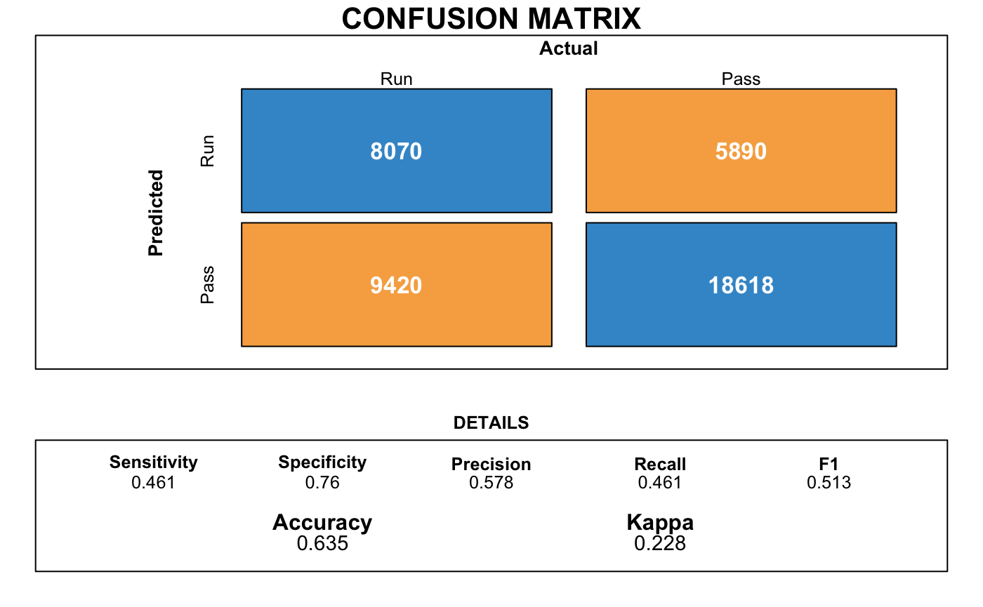
The accuracy of our predicted model is 63% ! Not bad but we can do better. Let’s try Naive Bayes, KNN, Decision Tree, Random Forest, & Kernal Support Vector Machine next.


